
The Engineer’s Guide to IGA: Decoding Isogeometric Analysis
By: A Fellow Math Enthusiast
Target Audience: Mechanical & Civil Engineers, CAD Specialists
Introduction: The “Mesh” Problem
If you have done Finite Element Analysis (FEA), you know the pain: you design a beautiful smooth curve in CAD, but to analyze it, you chop it into jagged little triangles (a mesh). You lose accuracy, and “remeshing” is a nightmare.
Isogeometric Analysis (IGA) solves this by asking: “Why don’t we just solve the differential equations directly on the smooth CAD geometry?”
The Syllabus Map
| Your Bachelor’s Subject | The IGA Implementation |
| Numerical Methods | B-Splines & NURBS (The Basis Functions) |
| Linear Algebra | Tensor Products (Building 3D from 1D) |
| Calculus II / III | Jacobians & Mapping (Real World vs. Parametric) |
| Differential Eqs | Weak Form / Galerkin Method (The Physics) |
| Computational Geometry | Knot Vectors (Controlling Smoothness) |
The Breakdown
- Numerical Methods (NURBS)
-
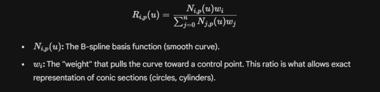
- The Component: In FEA, you use simple polynomials (lines, parabolas) to approximate shape. In IGA, you use Non-Uniform Rational B-Splines (NURBS). These are the exact mathematical functions used by SolidWorks or AutoCAD to draw curves.
- The Math: You are replacing the standard FEA basis functions N_i with B-spline basis functions R_i. If you understand how to interpolate a curve using control points, you understand the core of IGA.
- Linear Algebra (Tensor Products)
-
- The Component: How do you describe a 3D volume using 1D curves?
- The Math: You use Tensor Products. A 3D shape in IGA is often just the outer product of three 1D spline vectors.
- Basis(u,v,w) = N(u) \otimes M(v) \otimes L(w)
- This allows you to handle massive 3D matrices efficiently by breaking them down into 1D linear algebra operations.
- Calculus III (The Jacobian)
-
- The Component: Integration.
- The Math: To solve the physics, you must integrate over the volume. But IGA works in a “parametric space” (perfect squares). You use the Jacobian Determinant (from Calc III change of variables) to map the physics from the twisted “Real World” shape back to the perfect “Parametric” parent domain.

Comments :