
The Engineer’s Guide to Fractional Calculus: Decoding Non-Integer Derivatives

By: A Fellow Math Enthusiast
Target Audience: Control Systems Engineers, Material Scientists
Introduction: In Between Dimensions
You know the first derivative (velocity) and the second derivative (acceleration). But what is the half-derivative?
Fractional Calculus allows us to take the $0.5^{th}$ derivative. This is not just a math trick; it is the best way to model “memory” in materials, like viscoelastic polymers or batteries, where the current state depends on the entire history of the system.
The Syllabus Map
| Your Bachelor’s Subject | The Implementation |
| Calculus II | The Gamma Function (Factorials for fractions) |
| Complex Analysis | Cauchy Integral Formula (The definition) |
| Transform Calculus | Laplace Transforms (Solving the equations) |
| Diff Eqs | Convolution Integrals (Memory effects) |
| Series & Sequences | Power Series (Mittag-Leffler Function) |
The Breakdown
- Calculus II (The Gamma Function)
-
- The Component: Generalizing the factorial.
- The Math: The power rule \frac{d^n}{dx^n} x^k involves factorials (k!). To do this for non-integers, we replace the factorial with the Gamma Function \Gamma(z).
- This allows us to calculate things like \frac{d^{0.5}}{dx^{0.5}} x.
- Diff Eqs (Convolution)
-
- The Component: Memory.
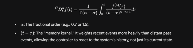
- The Math: Standard derivatives are “local” (slope right now). Fractional derivatives are “non-local.” They are defined by an integral (Riemann-Liouville definition) that sums up the function’s behavior from time t=0 to t=now. This is technically a Convolution, a concept you likely used in Signals and Systems.
- Transform Calculus (Laplace)
-
- The Component: Solving the system.
- The Math: Solving fractional differential equations in the time domain is hard. But in the Laplace Domain (s-domain), the fractional derivative $D^\alpha simply becomes multiplication by s^\alpha. You solve it algebraically, just like you did in Control Theory 101.

Comments :