
The Engineer’s Guide to QAOA: Decoding Quantum Algorithms

By: A Fellow Math Enthusiast
Target Audience: Optimization Engineers, Logistics Specialists
Introduction: Optimization on a Wave
The Quantum Approximate Optimization Algorithm (QAOA) is a leading candidate for using near-term quantum computers to solve massive combinatorial problems (like the Traveling Salesman or Portfolio Optimization). It mixes quantum mechanics with classical optimization.
The Syllabus Map
| Your Bachelor’s Subject | The QAOA Implementation |
| Linear Algebra | Unitary Matrices & Eigenvalues (The Gates) |
| Complex Numbers | Phase Angles (The Rotation) |
| Optimization | Expectation Values (The Cost Function) |
| Probability | Measurement & Collapse (The Output) |
| Physics / Mechanics | Hamiltonians (The Energy Landscape) |
The Breakdown
- Physics / Linear Algebra (Hamiltonians)
-
- The Component: Defining the problem.
- The Math: In quantum, we don’t write a “cost function” f(x). We write a matrix called a Hamiltonian (H_C). The “Eigenvalues” of this matrix are the possible costs, and the “Eigenvectors” are the possible solutions. We want to find the eigenvector with the lowest eigenvalue (Ground State).
- Complex Numbers (Unitary Evolution)
-
- The Component: The Algorithm.
- The Math: The algorithm applies rotations in a complex vector space.
- U(\gamma) = e^{-i \gamma H_C}
- This is Euler’s formula on steroids. You are rotating the state vector by an angle \gamma driven by the problem matrix H_C.
- Optimization (Classical Hybrid)
-
- The Component: Tuning the circuit.
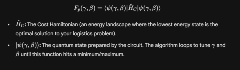
- The Math: QAOA doesn’t just run once. It outputs a quantum state, measures the “average energy” (Expectation Value \langle \psi | H_C | \psi \rangle), and feeds that number into a Classical Optimizer (like Gradient Descent) running on a normal laptop. The laptop tells the quantum computer to adjust the angles \gamma and \beta to try and get a lower energy next time.

Comments :